Representation of continuous time, periodic signals in the frequency domain.
Periodic signals occur frequently — motion of planets and their satellites, vibration of oscillators, electric power distribution, beating of the heart, vibration of vocal chords, etc.
Lecture #7:
CONTINUOUS TIME FOURIER SERIES FOR PERIODIC SIGNALS
Motivation:
Representation of continuous time, periodic signals in the frequency domain
Periodic signals occur frequently — motion of planets and their satellites, vibration of oscillators, electric power distribution, beating of the heart, vibration of vocal chords, etc.
Outline:
Fourier series of periodic functions
Examples of Fourier series — periodic impulse train
Fourier transforms of periodic functions — relation to Fourier series
Conclusions
I. FOURIER SERIES OF A PERIODIC FUNCTION
1/ Periodic time function
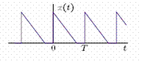
x(t) is a periodic time function with period T.
Such a periodic function can be expanded in an infinite series of exponential time functions called the Fourier series,
2/ Fourier series coefficients
The coefficients of the Fourier series can be found as follows.
The integral can be evaluated as follows.
The set of exponential time functions are said to be an orthonormal basis.
The coefficients are
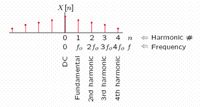
3/ Definition of line spectra, harmonics
The fundamental frequency fo = 1/T . The Fourier series coefficients plotted as a function of n or nfo is called a Fourier spectrum.
II. EXAMPLES OF FOURIER SERIES OF PERIODIC TIME FUNCTIONS
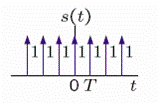
1/ Periodic impulse train
The periodic impulse train is an important periodic time function and we derive its Fourier series coefficients.
The Fourier series coefficients are found as follows
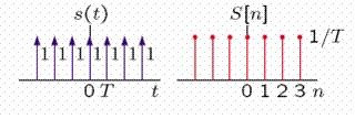
The Fourier series coefficients are
The time function and spectrum are shown below.
To summarize, the periodic impulse train can be represented by its Fourier series,
The Fourier series of the periodic impulse train is
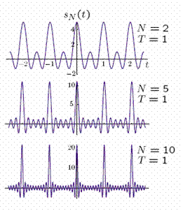
It is not obvious that the two expressions are equal. To investigate this, we define the partial sum of the Fourier series, sN(t),
and investigate its behavior as N →∞.
The partial sum of the Fourier series is
We can use the summation formula for a finite geometric series (Lecture 10) to sum this series,
Note that this function is periodic with period T, and
The first zero of sN(t) is at
Thus, as N → ∞, each lobe gets larger and narrower. To determine if each lobe acts as an impulse, we need to find its area.