6.2 Using the normal distribution

The shaded area in the following graph indicates the area to the right of x . This area is represented by the probability P ( X > x ). Normal tables, computers, and calculators provide or calculate the probability P ( X > x ).

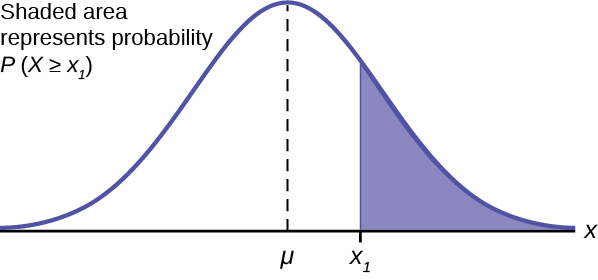
The area to the right is then P ( X > x ) = 1 – P ( X < x ). Remember, P ( X < x ) = Area to the left of the vertical line through x . P ( X < x ) = 1 – P ( X < x ) = Area to the right of the vertical line through x . P ( X < x ) is the same as P ( X ≤ x ) and P ( X > x ) is the same as P ( X ≥ x ) for continuous distributions.

Calculations of probabilities

To find the probability for probability density functions with a continuous random variable we need to calculate the area under the function across the values of X we are interested in. For the normal distribution this seems a difficult task given the complexity of the formula. There is, however, a simply way to get what we want. Here again is the formula for the normal distribution:

Looking at the formula for the normal distribution it is not clear just how we are going to solve for the probability doing it the same way we did it with the previous probability functions. There we put the data into the formula and did the math.

To solve this puzzle we start knowing that the area under a probability density function is the probability.

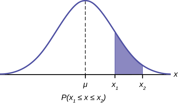
This shows that the area between X ₁ and X ₂ is the probability as stated in the formula: P (X ₁ ≤ x ≤ X ₂ )

The mathematical tool needed to find the area under a curve is integral calculus. The integral of the normal probability density function between the two points x ₁ and x ₂ is the area under the curve between these two points and is the probability between these two points.

Doing these integrals is no fun and can be very time consuming. But now, remembering that there are an infinite number of normal distributions out there, we can consider the one with a mean of zero and a standard deviation of 1. This particular normal distribution is given the name Standard Normal Distribution. Putting these values into the formula it reduces to a very simple equation. We can now quite easily calculate all probabilities for any value of x, for this particular normal distribution, that has a mean of zero and a standard deviation of 1. These have been produced and are available here in the text or everywhere on the web. They are presented in various ways. The table in this text is the most common presentation and is set up with probabilities for one-half the distribution beginning with zero, the mean, and moving outward. The shaded area in the graph at the top of the table represents the probability from zero to the specific Z value noted on the horizontal axis, Z.

The only problem is that even with this table, it would be a ridiculous coincidence that our data had a mean of zero and a standard deviation of one. The solution is to convert the distribution we have with its mean and standard deviation to this new Standard Normal Distribution. The Standard Normal has a random variable called Z.

Using the standard normal table, typically called the normal table, to find the probability of one standard deviation, go to the Z column, reading down to 1.0 and then read at column 0. That number, 0.3413 is the probability from zero to 1 standard deviation. At the top of the table is the shaded area in the distribution which is the probability for one standard deviation. The table has solved our integral calculus problem. But only if our data has a mean of zero and a standard deviation of 1.