To solve this equation numerically in a computer, the CT signals are discretized and the derivative is approximated.
2/ Forward Euler algorithm
a/ Discretization
Define
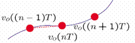
and approximate the derivative by the forward Euler algorithm
b/ Difference equation
Substituting the approximation for the derivative into the differential equation, we obtain
This equation can be written as a difference equation
This equation was solved iteratively for
and
to yield the solution
where α = T/RC. We now solve this difference equation using the Z-transform method.
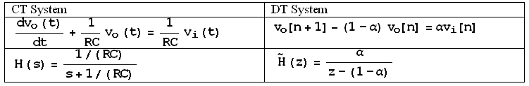
c/ System function
The Z-transform of the difference equation
is
so that the system function is
The region of convergence of
needs to be specified from the system description. Because we are simulating a CT system consisting of an RC circuit, we are dealing with a causal system, one that does not respond before it is stimulated. Then we know that the ROC is |z|>|1 − α|.
d/ Input and output Z-transforms
The input is
. Therefore,
Therefore,
This is a proper rational function and we expand it in a partial fraction expansion as follows
Because the ROC is outside a circle enclosing all the poles, the solution is
e/ Step response
CT and DT system step responses for α = T/RC, RC = 1,
The DT solution is increasingly accurate as T is made smaller. Note that when
T>2, the DT solution diverges. Why?
f/ Natural frequencies of the CT and DT systems
The natural frequency of the CT system is s = −1/(RC) and the natural frequency of the DT system is z = 1− α = 1− T/(RC) .
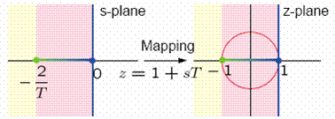
g/ Relation of natural frequencies in s- and z-planes
The CT system has a natural frequency of s = −1/RC and the DT system for the forward Euler algorithm has the natural frequency z = 1− (T/RC) = 1+sT . Thus, the forward Euler algorithm maps the s-plane into the z-plane by the mapping z = 1+sT . The mapping is shown below.
The conclusion is that for
, z<−1 and the DT approximation to the CT system is unstable. Therefore, to extend the range of stability, decrease T.
3/ Backward Euler algorithm
The forward Euler algorithm is one of many possible approximations to the derivative. Another is called the backward Euler algorithm.
a/ Discretization
Define
and approximate the derivative by the backward Euler algorithm
b/ Difference equation and system function
Substituting the approximation for the derivative into the differential equation as before, we now obtain